Building a content-based movie recommendation system using the MovieLens dataset
Introduction
In this project, we will build a movie recommendation system using content-based filtering. We will use the MovieLens dataset, provided in Kaggle, which contains movie and user data, to recommend movies to an user based on the genres of movies he has liked the most.
Resources
- GitHub repository containing this project and a list of dependencies

- Open this page in Google Colab

- Read the contents in my website
The video below contains an overview of the method we will implement. However, unlike the example above, they use a method which gives more weight to genres a user has rated more movies in. We will fix that mistake and show the differences in both methods.
Content-based filtering overview
The idea of content-based filtering is simple.
- represent items with a set of features
- discover a user’s preferences to each of those features, based on items they have already rated/consumed/liked that contain the features
- infer the user’s preference to unseen items based on those item features.
Unlike more sophisticated recommendation systems, such as collaborative filtering, content-based filtering only uses data provided by a single user to model their preferences. Thus it is much simpler to implement.
A concrete example
In our project, we will build a movie recommendation system, so let’s build an example using this theme. I will number the steps below and you can look for references to these tables in the Python implementation that comes right after.
-
We begin with a list of ratings a user has given to the movies they have watched.
Movie ID Movie Title User Rating 1 Inception 5.0 2 The Matrix 4.5 3 Interstellar 4.0 -
Each of the movies belongs to a list of genres.
Movie ID Movie Title Genres 1 Inception Sci-Fi, Thriller 2 The Matrix Sci-Fi, Action 3 Interstellar Sci-Fi, Drama -
If we average the ratings the user has given for each movie by genre, we get the user’s ratings for each genre.
- Sci-Fi appears in all three movies, so its average rating is: \(\frac{(5.0 + 4.5 + 4.0)}{3} = 4.5\)
- Thriller appears only in Inception, so its average rating is: 5.0
- Action appears only in The Matrix, so its average rating is: 4.5
- Drama appears only in Interstellar, so its average rating is: 4.0
This gives us the ratings by genre for that particular user.
Genre Average Rating Sci-Fi 4.5 Thriller 5.0 Action 4.5 Drama 4.0 In technical jargon, this is called the user profile and the component in your system that generates this is the user profiler.
-
Now, let’s consider a new list of movies this user has not yet watched.
Movie ID Movie Title Genres 4 Blade Runner 2049 Sci-Fi, Thriller 5 Mad Max: Fury Road Action, Sci-Fi 6 The Social Network Drama 7 The Crow Action, Horror 8 La La Land Musical, Romantic Comedy
When we select and preprocess item features, keeping them ready to match against user profiles, we performing content analysis. In our example, we use movie genres as their features, transforming them into what are called tags, and we are not considering other information such as the movie description, its release date or its director. Some of these could also be transformed into tags, while others need to be processed using NLP techniques.
-
To estimate the current user’s ratings for these unwatched movies, we take the average of the user’s ratings for the movie’s genres:
- Blade Runner 2049 (Sci-Fi, Thriller)
\(\frac{(4.5 + 5.0)}{2} = 4.75\) - Mad Max: Fury Road (Action, Sci-Fi)
\(\frac{(4.5 + 4.5)}{2} = 4.5\) - The Social Network (Drama)
- Drama’s average rating is 4.0, so the estimated rating is 4.0.
- The Crow (Action, Horror)
- Because the user has not ranked any horror movies yet, we can average over the ratings of the genres we do have. In this case, only Action, whose estimated rating is 4.5.
- La La Land (Musical, Romantic Comedy)
- The user has not rated any romantic comedies or musicals yet, so we are unable to estimate a rating for La La Land and thus we are unable to recommend it to this user.
Movie ID Movie Title Inferred Rating 4 Blade Runner 2049 4.75 5 Mad Max: Fury Road 4.5 6 The Social Network 4.0 7 The Crow 4.5 8 La La Land — - Blade Runner 2049 (Sci-Fi, Thriller)
Now we know that, if we were to recommend new movies for that user to watch, we would recommend “Blade Runner 2049” first, then “Mad Max: Fury Road” or “The Crow” and “The Social Network” last.
The process of selecting ranked items for a given users is called content retrieval.
Maybe we would like to prioritize “Mad Max: Fury Road” over “The Crow” since we have more user preference information to estimate the rating of the first movie, but that is not strictly necessary and we can consider them tied until the user rates more movies.
Downloading the dataset
As you have seen above, we need a dataset that contains:
- movies with their genres
- user ratings for movies
Fortunately, the MovieLens dataset has both of these pieces of data. We will download it using the kagglehub package.
import pathlib as pl

import kagglehub
import pandas as pd

(mvls_links_path, mvls_genometags_path, mvls_movies_path, mvls_genomescores_path, mvls_tags_path, mvls_ratings_path) = (
  list(pl.Path(kagglehub.dataset_download("grouplens/movielens-20m-dataset")).iterdir())
)
print(
  mvls_links_path, mvls_genometags_path, mvls_movies_path, mvls_genomescores_path, mvls_tags_path, mvls_ratings_path
)
/home/dodo/.cache/kagglehub/datasets/grouplens/movielens-20m-dataset/versions/1/link.csv /home/dodo/.cache/kagglehub/datasets/grouplens/movielens-20m-dataset/versions/1/genome_tags.csv /home/dodo/.cache/kagglehub/datasets/grouplens/movielens-20m-dataset/versions/1/movie.csv /home/dodo/.cache/kagglehub/datasets/grouplens/movielens-20m-dataset/versions/1/genome_scores.csv /home/dodo/.cache/kagglehub/datasets/grouplens/movielens-20m-dataset/versions/1/tag.csv /home/dodo/.cache/kagglehub/datasets/grouplens/movielens-20m-dataset/versions/1/rating.csv
MovieLens contains a collection of CSV files. You can see below the movie-related data, which contains the movie and year of release in one column, and all of its genres on another. This equivalent to table 2 in the example.
movies = pd.read_csv(mvls_movies_path).set_index("movieId").sort_index()
movies.head()
| title | genres | |
|---|---|---|
| movieId | ||
| 1 | Toy Story (1995) | Adventure|Animation|Children|Comedy|Fantasy |
| 2 | Jumanji (1995) | Adventure|Children|Fantasy |
| 3 | Grumpier Old Men (1995) | Comedy|Romance |
| 4 | Waiting to Exhale (1995) | Comedy|Drama|Romance |
| 5 | Father of the Bride Part II (1995) | Comedy |
The first thing we will do is represent movie genres by one-hot encoded columns. We will also keep a record of the names of these columns for later.
# get a single list of all unique genres for all movies
genres = list(set(movies["genres"].str.split("|").sum()))
genres = sorted(genres)
movies = movies.join(movies["genres"].str.get_dummies(sep="|")).drop("genres", axis=1)
print(f"Unique genres: {genres}")
print(f"Number of genres: {len(genres)}")
movies.head()
Unique genres: ['(no genres listed)', 'Action', 'Adventure', 'Animation', 'Children', 'Comedy', 'Crime', 'Documentary', 'Drama', 'Fantasy', 'Film-Noir', 'Horror', 'IMAX', 'Musical', 'Mystery', 'Romance', 'Sci-Fi', 'Thriller', 'War', 'Western']
Number of genres: 20
| title | (no genres listed) | Action | Adventure | Animation | Children | Comedy | Crime | Documentary | Drama | ... | Film-Noir | Horror | IMAX | Musical | Mystery | Romance | Sci-Fi | Thriller | War | Western | |
|---|---|---|---|---|---|---|---|---|---|---|---|---|---|---|---|---|---|---|---|---|---|
| movieId | |||||||||||||||||||||
| 1 | Toy Story (1995) | 0 | 0 | 1 | 1 | 1 | 1 | 0 | 0 | 0 | ... | 0 | 0 | 0 | 0 | 0 | 0 | 0 | 0 | 0 | 0 |
| 2 | Jumanji (1995) | 0 | 0 | 1 | 0 | 1 | 0 | 0 | 0 | 0 | ... | 0 | 0 | 0 | 0 | 0 | 0 | 0 | 0 | 0 | 0 |
| 3 | Grumpier Old Men (1995) | 0 | 0 | 0 | 0 | 0 | 1 | 0 | 0 | 0 | ... | 0 | 0 | 0 | 0 | 0 | 1 | 0 | 0 | 0 | 0 |
| 4 | Waiting to Exhale (1995) | 0 | 0 | 0 | 0 | 0 | 1 | 0 | 0 | 1 | ... | 0 | 0 | 0 | 0 | 0 | 1 | 0 | 0 | 0 | 0 |
| 5 | Father of the Bride Part II (1995) | 0 | 0 | 0 | 0 | 0 | 1 | 0 | 0 | 0 | ... | 0 | 0 | 0 | 0 | 0 | 0 | 0 | 0 | 0 | 0 |
5 rows × 21 columns
Regarding user ratings to movies, MovieLens provides us with 20 million ratings. In the cell below, you can see a few basic characteristics of user ratings. Most importantly, they range from 0.5 to 5 in intervals of 0.5
ratings = pd.read_csv(mvls_ratings_path)
ratings["rating"].value_counts()
rating
4.0    5561926
3.0    4291193
5.0    2898660
3.5    2200156
4.5    1534824
2.0    1430997
2.5     883398
1.0     680732
1.5     279252
0.5     239125
Name: count, dtype: int64
A user rating to a movie ties a user ID to a movie ID and contains the 0.5–5 rating the user has given the movie. In this project, we will work only with the user whose ID is 1. Let’s peek at some movies he has seen and their ratings.
We can see that user 1 has watched and rated 175 movies. That is a lot of movies. Also, the minimum rating user 1 has given to a movie is 3, far from the 0.5 it is allowed to give.
user_ratings = ratings[ratings["userId"] == 1]
ax = user_ratings["rating"].hist(bins=10, range=(0, 5))
ax.bar_label(ax.containers[0]);
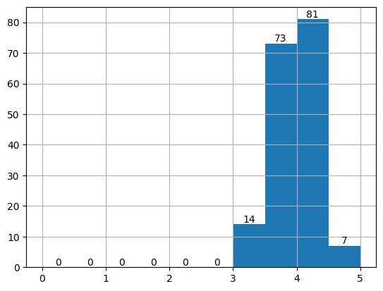
This is what the user-movie rating data actually looks like. This is equivalent to table 1 in the example.
user_ratings.head()
| userId | movieId | rating | timestamp | |
|---|---|---|---|---|
| 0 | 1 | 2 | 3.5 | 2005-04-02 23:53:47 |
| 1 | 1 | 29 | 3.5 | 2005-04-02 23:31:16 |
| 2 | 1 | 32 | 3.5 | 2005-04-02 23:33:39 |
| 3 | 1 | 47 | 3.5 | 2005-04-02 23:32:07 |
| 4 | 1 | 50 | 3.5 | 2005-04-02 23:29:40 |
Computing user-genre preferences
Our goal now will be to generate the user’s features, which will be derived from the genres of the movies they have watched and their ratings.
To make things easier for us, we will join user 1’s movie ratings with the genres of those movies.
user_ratings = user_ratings[["userId", "movieId", "rating"]].merge(movies, on="movieId")
user_ratings.head()
| userId | movieId | rating | title | (no genres listed) | Action | Adventure | Animation | Children | Comedy | ... | Film-Noir | Horror | IMAX | Musical | Mystery | Romance | Sci-Fi | Thriller | War | Western | |
|---|---|---|---|---|---|---|---|---|---|---|---|---|---|---|---|---|---|---|---|---|---|
| 0 | 1 | 2 | 3.5 | Jumanji (1995) | 0 | 0 | 1 | 0 | 1 | 0 | ... | 0 | 0 | 0 | 0 | 0 | 0 | 0 | 0 | 0 | 0 |
| 1 | 1 | 29 | 3.5 | City of Lost Children, The (Cité des enfants p... | 0 | 0 | 1 | 0 | 0 | 0 | ... | 0 | 0 | 0 | 0 | 1 | 0 | 1 | 0 | 0 | 0 |
| 2 | 1 | 32 | 3.5 | Twelve Monkeys (a.k.a. 12 Monkeys) (1995) | 0 | 0 | 0 | 0 | 0 | 0 | ... | 0 | 0 | 0 | 0 | 1 | 0 | 1 | 1 | 0 | 0 |
| 3 | 1 | 47 | 3.5 | Seven (a.k.a. Se7en) (1995) | 0 | 0 | 0 | 0 | 0 | 0 | ... | 0 | 0 | 0 | 0 | 1 | 0 | 0 | 1 | 0 | 0 |
| 4 | 1 | 50 | 3.5 | Usual Suspects, The (1995) | 0 | 0 | 0 | 0 | 0 | 0 | ... | 0 | 0 | 0 | 0 | 1 | 0 | 0 | 1 | 0 | 0 |
5 rows × 24 columns
Now, we will propagate the user’s ratings to the genres of each movie. by multiplying the ratings user 1 has given to a movie with the genre columns of each movie. You will see that the one-hot encoding of that movie will become the actual ratings user 1 has given to the movie.
# multiply the genre columns by the rating
user_ratings[genres] = user_ratings[genres].multiply(user_ratings["rating"], axis="index")
user_ratings.head()
| userId | movieId | rating | title | (no genres listed) | Action | Adventure | Animation | Children | Comedy | ... | Film-Noir | Horror | IMAX | Musical | Mystery | Romance | Sci-Fi | Thriller | War | Western | |
|---|---|---|---|---|---|---|---|---|---|---|---|---|---|---|---|---|---|---|---|---|---|
| 0 | 1 | 2 | 3.5 | Jumanji (1995) | 0.0 | 0.0 | 3.5 | 0.0 | 3.5 | 0.0 | ... | 0.0 | 0.0 | 0.0 | 0.0 | 0.0 | 0.0 | 0.0 | 0.0 | 0.0 | 0.0 |
| 1 | 1 | 29 | 3.5 | City of Lost Children, The (Cité des enfants p... | 0.0 | 0.0 | 3.5 | 0.0 | 0.0 | 0.0 | ... | 0.0 | 0.0 | 0.0 | 0.0 | 3.5 | 0.0 | 3.5 | 0.0 | 0.0 | 0.0 |
| 2 | 1 | 32 | 3.5 | Twelve Monkeys (a.k.a. 12 Monkeys) (1995) | 0.0 | 0.0 | 0.0 | 0.0 | 0.0 | 0.0 | ... | 0.0 | 0.0 | 0.0 | 0.0 | 3.5 | 0.0 | 3.5 | 3.5 | 0.0 | 0.0 |
| 3 | 1 | 47 | 3.5 | Seven (a.k.a. Se7en) (1995) | 0.0 | 0.0 | 0.0 | 0.0 | 0.0 | 0.0 | ... | 0.0 | 0.0 | 0.0 | 0.0 | 3.5 | 0.0 | 0.0 | 3.5 | 0.0 | 0.0 |
| 4 | 1 | 50 | 3.5 | Usual Suspects, The (1995) | 0.0 | 0.0 | 0.0 | 0.0 | 0.0 | 0.0 | ... | 0.0 | 0.0 | 0.0 | 0.0 | 3.5 | 0.0 | 0.0 | 3.5 | 0.0 | 0.0 |
5 rows × 24 columns
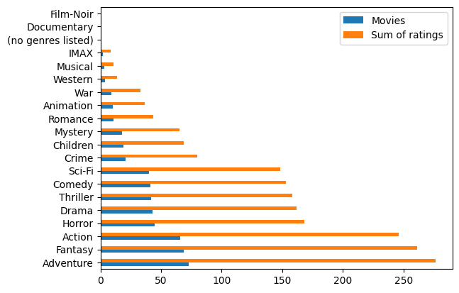
Now, if we sum all the ratings user 1 has given to the movies they have watched by genre, we get a proxy value that denotes how much user 1 enjoys each of the genres.
user_genre_preferences = pd.DataFrame(
  data={"Movies": (user_ratings[genres] != 0).sum(), "Sum of ratings": user_ratings[genres].sum()}
)
user_genre_preferences.sort_values("Sum of ratings", ascending=False)
| Movies | Sum of ratings | |
|---|---|---|
| Adventure | 73 | 276.5 |
| Fantasy | 69 | 261.5 |
| Action | 66 | 246.0 |
| Horror | 45 | 168.5 |
| Drama | 43 | 162.0 |
| Thriller | 42 | 158.0 |
| Comedy | 41 | 153.0 |
| Sci-Fi | 40 | 148.5 |
| Crime | 21 | 80.0 |
| Children | 19 | 68.5 |
| Mystery | 18 | 65.0 |
| Romance | 11 | 43.5 |
| Animation | 10 | 36.5 |
| War | 9 | 33.0 |
| Western | 4 | 13.5 |
| Musical | 3 | 11.0 |
| IMAX | 2 | 8.5 |
| (no genres listed) | 0 | 0.0 |
| Documentary | 0 | 0.0 |
| Film-Noir | 0 | 0.0 |
Because the magnitudes of these sums of ratings can get out of hand, we can divide them by the sum of all ratings and get neat values that all add up to 1.
user_genre_preferences["Normalized sum of ratings"] = (
  user_genre_preferences["Sum of ratings"] / user_genre_preferences["Sum of ratings"].max()
)
user_genre_preferences.sort_values("Normalized sum of ratings", ascending=False)
| Movies | Sum of ratings | Normalized sum of ratings | |
|---|---|---|---|
| Adventure | 73 | 276.5 | 1.000000 |
| Fantasy | 69 | 261.5 | 0.945750 |
| Action | 66 | 246.0 | 0.889693 |
| Horror | 45 | 168.5 | 0.609403 |
| Drama | 43 | 162.0 | 0.585895 |
| Thriller | 42 | 158.0 | 0.571429 |
| Comedy | 41 | 153.0 | 0.553345 |
| Sci-Fi | 40 | 148.5 | 0.537071 |
| Crime | 21 | 80.0 | 0.289331 |
| Children | 19 | 68.5 | 0.247740 |
| Mystery | 18 | 65.0 | 0.235081 |
| Romance | 11 | 43.5 | 0.157324 |
| Animation | 10 | 36.5 | 0.132007 |
| War | 9 | 33.0 | 0.119349 |
| Western | 4 | 13.5 | 0.048825 |
| Musical | 3 | 11.0 | 0.039783 |
| IMAX | 2 | 8.5 | 0.030741 |
| (no genres listed) | 0 | 0.0 | 0.000000 |
| Documentary | 0 | 0.0 | 0.000000 |
| Film-Noir | 0 | 0.0 | 0.000000 |
These values are interesting and they may be used as an indication of how much a user prefers certain movie genres. This is the way that is taught in the video at the beginning of the page.
However, because this method just sums all ratings the user has given to a collection of movies, it favors those genres in which the user has given more ratings, regardless of how low the ratings are.
For example, if a user watches 9 action movies and gives a rating of 1 to all of them, the Action genre will have a weight of 9 in our preference vector:
1 + 1 + 1 + 1 + 1 + 1 + 1 + 1 + 1 = 9
If that same user watches 2 musicals (I know, who likes musicals) but gives a rating of 4 to both of them, the Musical genre will have a weight of 8 in our fetaure vector, which is less than the weight of the Action genre.
4 + 4 = 8
But we can clearly see that this user hates action movies but loves musicals!
Our hypothesis is corroborated in the chart below, in which our sum of ratings for a genre grows as the user watches more movies.
user_genre_preferences[["Movies", "Sum of ratings"]].sort_values("Movies", ascending=False).plot.barh()
<Axes: >
By looking at the correlations between number of movies watched, sum of ratings and the normalized sum of ratings, we can see a pretty hgh positive correlation between all of them.
user_genre_preferences.corr()
| Movies | Sum of ratings | Normalized sum of ratings | |
|---|---|---|---|
| Movies | 1.000000 | 0.999871 | 0.999871 |
| Sum of ratings | 0.999871 | 1.000000 | 1.000000 |
| Normalized sum of ratings | 0.999871 | 1.000000 | 1.000000 |
One way we can mitigate this is by taking the average of the ratings a user gives to the movies of a particular genre as their preference for that genre. The table below is the one presented in step 3 of the example.
user_genre_preferences["Normalized by movies in genre"] = (
  user_genre_preferences["Sum of ratings"] / user_genre_preferences["Movies"]
).fillna(0)
user_genre_preferences = user_genre_preferences.sort_values("Normalized by movies in genre", ascending=False)
user_genre_preferences
| Movies | Sum of ratings | Normalized sum of ratings | Normalized by movies in genre | |
|---|---|---|---|---|
| IMAX | 2 | 8.5 | 0.030741 | 4.250000 |
| Romance | 11 | 43.5 | 0.157324 | 3.954545 |
| Crime | 21 | 80.0 | 0.289331 | 3.809524 |
| Fantasy | 69 | 261.5 | 0.945750 | 3.789855 |
| Adventure | 73 | 276.5 | 1.000000 | 3.787671 |
| Drama | 43 | 162.0 | 0.585895 | 3.767442 |
| Thriller | 42 | 158.0 | 0.571429 | 3.761905 |
| Horror | 45 | 168.5 | 0.609403 | 3.744444 |
| Comedy | 41 | 153.0 | 0.553345 | 3.731707 |
| Action | 66 | 246.0 | 0.889693 | 3.727273 |
| Sci-Fi | 40 | 148.5 | 0.537071 | 3.712500 |
| War | 9 | 33.0 | 0.119349 | 3.666667 |
| Musical | 3 | 11.0 | 0.039783 | 3.666667 |
| Animation | 10 | 36.5 | 0.132007 | 3.650000 |
| Mystery | 18 | 65.0 | 0.235081 | 3.611111 |
| Children | 19 | 68.5 | 0.247740 | 3.605263 |
| Western | 4 | 13.5 | 0.048825 | 3.375000 |
| (no genres listed) | 0 | 0.0 | 0.000000 | 0.000000 |
| Documentary | 0 | 0.0 | 0.000000 | 0.000000 |
| Film-Noir | 0 | 0.0 | 0.000000 | 0.000000 |
If we now look at the correlation of the two feature sets implemented, we can see they are mostly uncorrelated, which means they are two completely different ways of expressing user preference.
user_genre_preferences[["Normalized sum of ratings", "Normalized by movies in genre"]].corr()
| Normalized sum of ratings | Normalized by movies in genre | |
|---|---|---|
| Normalized sum of ratings | 1.000000 | 0.451363 |
| Normalized by movies in genre | 0.451363 | 1.000000 |
As you can see above, the second choice of features is very interesting. While before, we thought that the user enjoyed the Adventure, Fantasy Action and Horror genres, now we belive they enjoy IMAX movies, romances and crimes, even though they have watched less movies in that genre.
One thing to note is that not all genres have inferred ratings for the given user. In cases where the user has not rated any movie of a particular genre, that genre will not have a rating. In our case, since MovieLens ratings start at 0.5, we use 0 to denote the absence of ratings.
genres_with_ratings = (user_genre_preferences["Normalized by movies in genre"] > 0).sum()
genres_without_ratings = len(user_genre_preferences) - genres_with_ratings

print(f"Total genres: {len(user_genre_preferences)}\nNumber of genres with ratings for user: {genres_with_ratings}")
Total genres: 20
Number of genres with ratings for user: 17
Inferring preferences for unwatched movies
Now that we know how much the user prefers each genre, we will compute the ratings for movies that user has not watched yet.
First, let’s get all the movies they have not watched from MovieLens. This would be the table from step 4 in the example.
# get the movies that the user has not seen
unwatched_movies = movies.loc[~movies.index.isin(user_ratings["movieId"])].copy()
unwatched_movies
| title | (no genres listed) | Action | Adventure | Animation | Children | Comedy | Crime | Documentary | Drama | ... | Film-Noir | Horror | IMAX | Musical | Mystery | Romance | Sci-Fi | Thriller | War | Western | |
|---|---|---|---|---|---|---|---|---|---|---|---|---|---|---|---|---|---|---|---|---|---|
| movieId | |||||||||||||||||||||
| 1 | Toy Story (1995) | 0 | 0 | 1 | 1 | 1 | 1 | 0 | 0 | 0 | ... | 0 | 0 | 0 | 0 | 0 | 0 | 0 | 0 | 0 | 0 |
| 3 | Grumpier Old Men (1995) | 0 | 0 | 0 | 0 | 0 | 1 | 0 | 0 | 0 | ... | 0 | 0 | 0 | 0 | 0 | 1 | 0 | 0 | 0 | 0 |
| 4 | Waiting to Exhale (1995) | 0 | 0 | 0 | 0 | 0 | 1 | 0 | 0 | 1 | ... | 0 | 0 | 0 | 0 | 0 | 1 | 0 | 0 | 0 | 0 |
| 5 | Father of the Bride Part II (1995) | 0 | 0 | 0 | 0 | 0 | 1 | 0 | 0 | 0 | ... | 0 | 0 | 0 | 0 | 0 | 0 | 0 | 0 | 0 | 0 |
| 6 | Heat (1995) | 0 | 1 | 0 | 0 | 0 | 0 | 1 | 0 | 0 | ... | 0 | 0 | 0 | 0 | 0 | 0 | 0 | 1 | 0 | 0 |
| ... | ... | ... | ... | ... | ... | ... | ... | ... | ... | ... | ... | ... | ... | ... | ... | ... | ... | ... | ... | ... | ... |
| 131254 | Kein Bund für's Leben (2007) | 0 | 0 | 0 | 0 | 0 | 1 | 0 | 0 | 0 | ... | 0 | 0 | 0 | 0 | 0 | 0 | 0 | 0 | 0 | 0 |
| 131256 | Feuer, Eis & Dosenbier (2002) | 0 | 0 | 0 | 0 | 0 | 1 | 0 | 0 | 0 | ... | 0 | 0 | 0 | 0 | 0 | 0 | 0 | 0 | 0 | 0 |
| 131258 | The Pirates (2014) | 0 | 0 | 1 | 0 | 0 | 0 | 0 | 0 | 0 | ... | 0 | 0 | 0 | 0 | 0 | 0 | 0 | 0 | 0 | 0 |
| 131260 | Rentun Ruusu (2001) | 1 | 0 | 0 | 0 | 0 | 0 | 0 | 0 | 0 | ... | 0 | 0 | 0 | 0 | 0 | 0 | 0 | 0 | 0 | 0 |
| 131262 | Innocence (2014) | 0 | 0 | 1 | 0 | 0 | 0 | 0 | 0 | 0 | ... | 0 | 1 | 0 | 0 | 0 | 0 | 0 | 0 | 0 | 0 |
27103 rows × 21 columns
As an intermediate step, we will to propagate the user’s genre preferences to the preferences of these unwatched movies.
movie_genre_ratings = unwatched_movies[genres].multiply(user_genre_preferences["Normalized by movies in genre"])
movie_genre_ratings
| (no genres listed) | Action | Adventure | Animation | Children | Comedy | Crime | Documentary | Drama | Fantasy | Film-Noir | Horror | IMAX | Musical | Mystery | Romance | Sci-Fi | Thriller | War | Western | |
|---|---|---|---|---|---|---|---|---|---|---|---|---|---|---|---|---|---|---|---|---|
| movieId | ||||||||||||||||||||
| 1 | 0.0 | 0.000000 | 3.787671 | 3.65 | 3.605263 | 3.731707 | 0.000000 | 0.0 | 0.000000 | 3.789855 | 0.0 | 0.000000 | 0.0 | 0.0 | 0.0 | 0.000000 | 0.0 | 0.000000 | 0.0 | 0.0 |
| 3 | 0.0 | 0.000000 | 0.000000 | 0.00 | 0.000000 | 3.731707 | 0.000000 | 0.0 | 0.000000 | 0.000000 | 0.0 | 0.000000 | 0.0 | 0.0 | 0.0 | 3.954545 | 0.0 | 0.000000 | 0.0 | 0.0 |
| 4 | 0.0 | 0.000000 | 0.000000 | 0.00 | 0.000000 | 3.731707 | 0.000000 | 0.0 | 3.767442 | 0.000000 | 0.0 | 0.000000 | 0.0 | 0.0 | 0.0 | 3.954545 | 0.0 | 0.000000 | 0.0 | 0.0 |
| 5 | 0.0 | 0.000000 | 0.000000 | 0.00 | 0.000000 | 3.731707 | 0.000000 | 0.0 | 0.000000 | 0.000000 | 0.0 | 0.000000 | 0.0 | 0.0 | 0.0 | 0.000000 | 0.0 | 0.000000 | 0.0 | 0.0 |
| 6 | 0.0 | 3.727273 | 0.000000 | 0.00 | 0.000000 | 0.000000 | 3.809524 | 0.0 | 0.000000 | 0.000000 | 0.0 | 0.000000 | 0.0 | 0.0 | 0.0 | 0.000000 | 0.0 | 3.761905 | 0.0 | 0.0 |
| ... | ... | ... | ... | ... | ... | ... | ... | ... | ... | ... | ... | ... | ... | ... | ... | ... | ... | ... | ... | ... |
| 131254 | 0.0 | 0.000000 | 0.000000 | 0.00 | 0.000000 | 3.731707 | 0.000000 | 0.0 | 0.000000 | 0.000000 | 0.0 | 0.000000 | 0.0 | 0.0 | 0.0 | 0.000000 | 0.0 | 0.000000 | 0.0 | 0.0 |
| 131256 | 0.0 | 0.000000 | 0.000000 | 0.00 | 0.000000 | 3.731707 | 0.000000 | 0.0 | 0.000000 | 0.000000 | 0.0 | 0.000000 | 0.0 | 0.0 | 0.0 | 0.000000 | 0.0 | 0.000000 | 0.0 | 0.0 |
| 131258 | 0.0 | 0.000000 | 3.787671 | 0.00 | 0.000000 | 0.000000 | 0.000000 | 0.0 | 0.000000 | 0.000000 | 0.0 | 0.000000 | 0.0 | 0.0 | 0.0 | 0.000000 | 0.0 | 0.000000 | 0.0 | 0.0 |
| 131260 | 0.0 | 0.000000 | 0.000000 | 0.00 | 0.000000 | 0.000000 | 0.000000 | 0.0 | 0.000000 | 0.000000 | 0.0 | 0.000000 | 0.0 | 0.0 | 0.0 | 0.000000 | 0.0 | 0.000000 | 0.0 | 0.0 |
| 131262 | 0.0 | 0.000000 | 3.787671 | 0.00 | 0.000000 | 0.000000 | 0.000000 | 0.0 | 0.000000 | 3.789855 | 0.0 | 3.744444 | 0.0 | 0.0 | 0.0 | 0.000000 | 0.0 | 0.000000 | 0.0 | 0.0 |
27103 rows × 20 columns
We then sum these preferences by movie and divide by the number of genres each movie has, to get the user preferences for each unwatched movie.
If we sort the movies by these inferred preferences, we get a list in descending order of the movies user 1 has not seen but might enjoy, based on their genres and the ratings user 1 has given to the movies they have seen.
denominator = movie_genre_ratings != 0
numerator = movie_genre_ratings.sum(axis=1)
content_based_ratings = numerator / denominator.sum(axis=1)
unwatched_movies["content_based_rating"] = content_based_ratings
unwatched_movies[["title", "content_based_rating"]].sort_values("content_based_rating", ascending=False)
| title | content_based_rating | |
|---|---|---|
| movieId | ||
| 4858 | Hail Columbia! (1982) | 4.25 |
| 4861 | Mission to Mir (1997) | 4.25 |
| 4459 | Alaska: Spirit of the Wild (1997) | 4.25 |
| 4460 | Encounter in the Third Dimension (1999) | 4.25 |
| 4461 | Siegfried & Roy: The Magic Box (1999) | 4.25 |
| ... | ... | ... |
| 131108 | The Fearless Four (1997) | NaN |
| 131110 | A House of Secrets: Exploring 'Dragonwyck' (2008) | NaN |
| 131166 | WWII IN HD (2009) | NaN |
| 131172 | Closed Curtain (2013) | NaN |
| 131260 | Rentun Ruusu (2001) | NaN |
27103 rows × 2 columns
Notice that this step already takes care of situations in which a movie belongs to a certain genre but the user has no rating for that genre. For example, this user has a rating for the Action gente, but not for Western. If movie belongs to both genres, the average will be taken only over one genre, since content_based_ratings.loc[movie_id, "<genre without user rating>"] will be equal to 0 and ignored when accounting for our denominator.
We can also compute the alternate user-genre preferences, using normalized sums of ratings, which are highly correlated with the number of movies watched in each genre. You can see we get a different list of movies, although some movies remain in the list and the first movie is the same.
content_based_ratings = unwatched_movies[genres].multiply(user_genre_preferences["Normalized sum of ratings"])
content_based_ratings = content_based_ratings.sum(axis=1)
unwatched_movies["content_based_rating2"] = content_based_ratings
unwatched_movies[["title", "content_based_rating2"]].sort_values("content_based_rating2", ascending=False)
| title | content_based_rating2 | |
|---|---|---|
| movieId | ||
| 81132 | Rubber (2010) | 4.783002 |
| 49593 | She (1965) | 4.725136 |
| 5018 | Motorama (1991) | 4.717902 |
| 71999 | Aelita: The Queen of Mars (Aelita) (1924) | 4.687161 |
| 72165 | Cirque du Freak: The Vampire's Assistant (2009) | 4.569620 |
| ... | ... | ... |
| 100246 | Pretty Sweet (2012) | 0.000000 |
| 99 | Heidi Fleiss: Hollywood Madam (1995) | 0.000000 |
| 100266 | Day Is Done (2011) | 0.000000 |
| 100287 | Head Games (2012) | 0.000000 |
| 96842 | Behind the Burly Q: The Story of Burlesque in ... | 0.000000 |
27103 rows × 2 columns
Both of the tables above are equivalent to the table presented in step 5 of the example.
Discussion
One disadvantage of content-based filtering is that we can only recommend an item for a user if that user has rated at least one other item that contains at least one feature in common with the item in question.
In our case, we can only recommend movies to a user if that movie contains at least one genre in common with another movie that the user has already rated.
The fewer features an unrated item has with rated ones, the less granular its inferred rating will be.
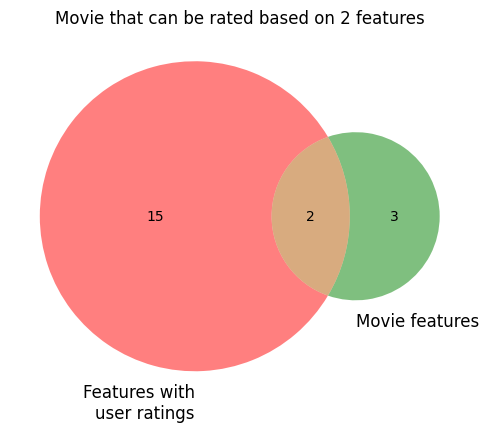
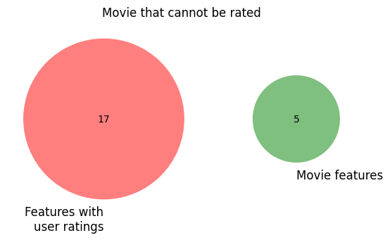
The diagrams below illustrate a situation in which a user has ratings for 17 genres, computed from the ratings of movies that contain those genres. In the first example, a movie with 5 genres has 2 genres in common with rated genres for the user, so we can compute an inferred rating for the movie.
In the second example, a movie with 5 genres has 0 genres in common with the rated genres for the user, so we cannot directly compute an inferred rating for it.
from matplotlib_venn import venn2
import matplotlib.pyplot as plt

movie_genres_count = 5
intersection = 2
set1 = genres_with_ratings - intersection
set2 = movie_genres_count - intersection
venn2(subsets=(set1, set2, intersection), set_labels=("Features with\nuser ratings", "Movie features"), alpha=0.5)
plt.title(f"Movie that can be rated based on {intersection} features")
plt.show()
venn2(
  subsets=(genres_with_ratings, movie_genres_count, 0),
  set_labels=("Features with\nuser ratings", "Movie features"),
  alpha=0.5,
)
plt.title("Movie that cannot be rated")
plt.show()
Because in our example, this user has watched over 100 movies, we are able to recommend over 90% of unwatched movies to them.
movies_with_inferred_ratings = (~unwatched_movies["content_based_rating"].isna()).sum()
print(f"Number of unwatched movies: {len(unwatched_movies)}")
print(f"Number of unwatched movies with inferred ratings: {movies_with_inferred_ratings}")
print(
  f"Percentage of unwatched movies with inferred ratings: {movies_with_inferred_ratings / len(unwatched_movies):.2%}"
)
Number of unwatched movies: 27103
Number of unwatched movies with inferred ratings: 24901
Percentage of unwatched movies with inferred ratings: 91.88%
Another disadvantage is that, depending on the number of features and technique employed in computing inferred ratings, the granularity of ratings can be very poor.
In our case, although we inferred ratings for over 24,000 movies, over 50% of them received one of 10 ratings.
inferred_ratings_count = unwatched_movies["content_based_rating"].value_counts()
topk = 10

print(f"Unique inferred ratings: {len(inferred_ratings_count)}")
print(
  f"Percentage of unwatched movies in the top {topk} inferred ratings: {(inferred_ratings_count.iloc[:topk].sum() / movies_with_inferred_ratings):.2%}"
)
Unique inferred ratings: 1182
Percentage of unwatched movies in the top 10 inferred ratings: 51.42%
This happens because, while we have \(n\) total features to represent user taste and items (the movie genres), the current user only has ratings for a subset \(m \leq n\) of the features.
Using a simple average over genre ratings, a movie’s inferred rating can only come from one of \(2^m-1\) possible values.
If the number of genres of the movie is known, say \(k\), then this value is restricted to \(\binom{m}{k}\), assuming that each possible rating is different.
The table below shows the number of possible ratings a movie may have, given the number of genres it has.
from scipy.special import comb

genres_count = unwatched_movies[genres].sum(axis=1).value_counts()
possible_ratings = pd.DataFrame(
  index=genres_count.index,
  data={
    "Number of Movies": genres_count,
    "Possible ratings": [comb(genres_with_ratings, i) for i in genres_count.index],
  },
)
possible_ratings["Movies per possible rating"] = (
  possible_ratings["Number of Movies"] / possible_ratings["Possible ratings"]
)
possible_ratings.index.name = "Number of genres"
possible_ratings
| Number of Movies | Possible ratings | Movies per possible rating | |
|---|---|---|---|
| Number of genres | |||
| 1 | 10816 | 17.0 | 636.235294 |
| 2 | 8766 | 136.0 | 64.455882 |
| 3 | 5260 | 680.0 | 7.735294 |
| 4 | 1685 | 2380.0 | 0.707983 |
| 5 | 468 | 6188.0 | 0.075630 |
| 6 | 82 | 12376.0 | 0.006626 |
| 7 | 20 | 19448.0 | 0.001028 |
| 8 | 5 | 24310.0 | 0.000206 |
| 10 | 1 | 19448.0 | 0.000051 |
Conclusion
In this project, we have built a movie recommendation system based on content-based filtering.
We went through the theory of content-based filtering as well as an example, then used a publicly available dataset to implement the system. We compared two ways of building user features and saw one of the downsides of content-based filtering, which is the inability of recommending new items to a user if those items don’t have intersecting features with the items the user has already rated.
See you guys next time!
Enjoy Reading This Article?
Here are some more articles you might like to read next: